03 - Heightmaps

In this article we talk about using a python notebook to generate a mesh from a heightmap and a color image. The heightmaps can either be for planar surfaces, or curved surfaces. Heightmaps and color images for curved surfaces should be equirectangular projections of a portion of a sphere. Here we an example of both a curved and a planar mesh, both of which are based off of the following graphic from http://chipcarroll.samexhibit.com/3d. This notebook is included in versions 1.01 or later of the modulesbuilder that can be downloaded from Getting Started.

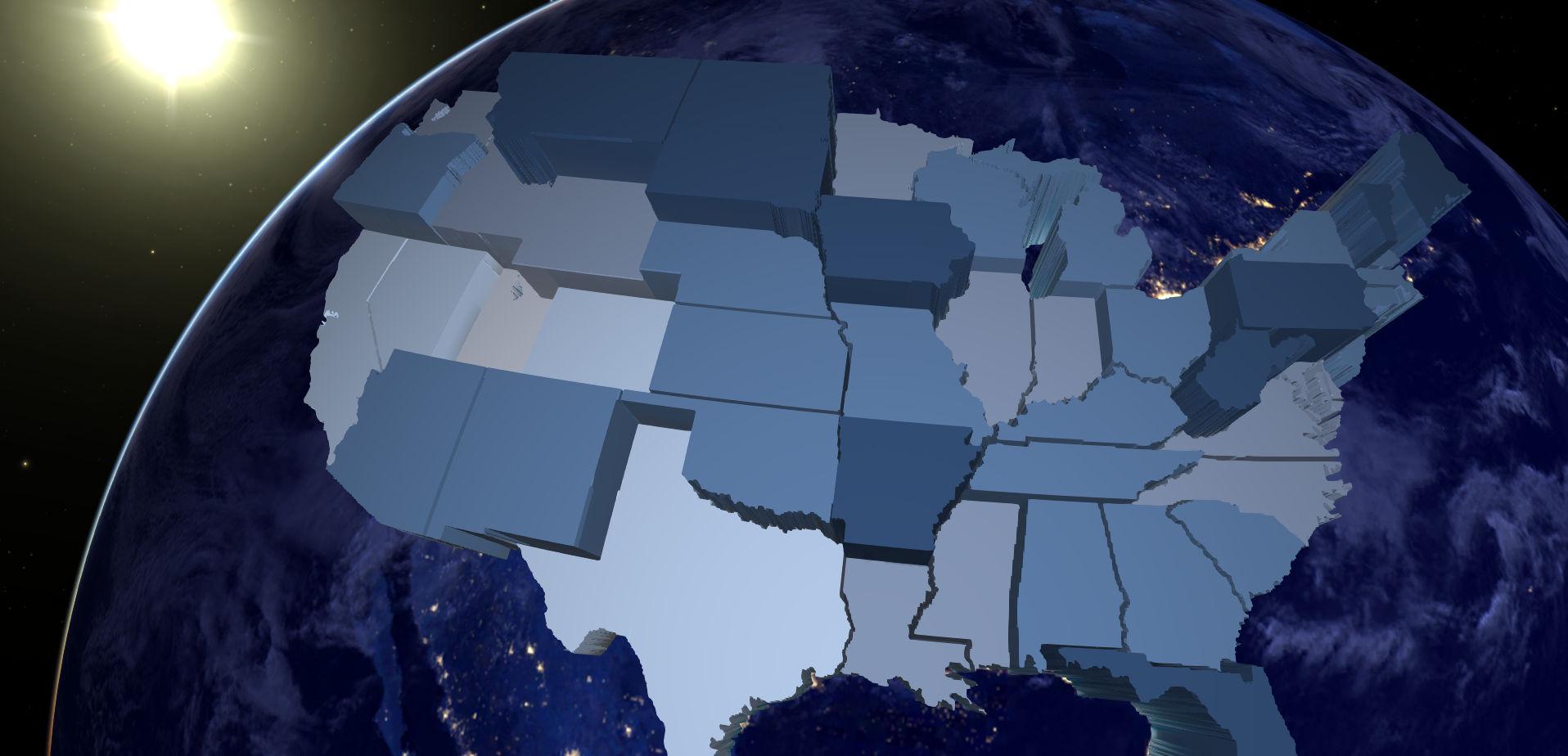
Mesh Properties:

There are many properties unique to the curved and planar meshes that can be changed in the notebook. These are set using functions in the fourth code cell of the notebook. This code cell also sets the standard scene, module information, and orbital object properties as in Spice Kernels with a few changes. Instead of using a spice or kepler file for the scene we define, we use a surface position file. This specifies a surface scene on the surface of a planet from the planet's name, a longitude, a latitude, and an altitude. Here our scene is 750km above the Continental United States. We also use "setsurfacepositionerrotation" to set the heading, pitch and roll of the surface positioned scene. We disable the planar mesh on start up by using the "showatstartup" function with the argument of "False". Finally, we align the curved mesh with the rotating Earth using the "setspicerotation" function. This just leaves curved mesh and planar mesh specific properties.

We defined two types of mesh objects earlier in the notebook, "PlanarMesh" and "CurvedMesh". These represent the planar and curved meshes with heightmaps. Both types of meshes take an orbital object when instantiated and both types of meshes have functions that set the properties of the mesh. Some of these properties are shared between both types of meshes, and some only apply to one type of mesh.

Shared Properties:

• setHeightmap: This sets the heightmap file for the mesh. The file should be located in the data folder or a directory, and this function should be passed the file's path relative to the data folder. The sizes of the deformations of the mesh are based on the data in this file and the heightmap scale. Planar meshes are deformed in the z-direction and curved meshes are deformed radially.
• setColorTex: This sets the color image file for the mesh. The file should be located in the data folder or a directory, and this function should be passed the file's path relative to the data folder.
• setMeshResolution: This sets the resolution of the mesh. For planar meshes, the first argument is the number of vertices along the x-direction and the second argument is the number of vertices along the y-direction. For curved meshes, the first argument is the number of vertices along the longitudinal direction and the second argument is the number of vertices along the latitudinal direction.
• setHightmapScale: This sets the size of the deformations due to the heightmap. The first argument is the deformation size if the heightmap has a value of 0. The second argument is the deformation size if the heightmap has a value of 1. The deformations of heightmap values between 0 and 1 are calculated using linear interpolation. This can be changed at run-time in the state manager under the name "heightmapScale"[check this]
• setHeightmapVerticalInvert / setColorVerticalInvert: Due to differing texture coordinate conventions, it is possible that your heightmap or color image or both could be upside down. Passing "True" to these functions will flip the vertical texture coordinate of the heightmap or color image respectively. This allows you to turn upside down images or heightmaps right-side up with minimal effort.

Curved Mesh Properties:

• setRadius: This sets the base radius for the curved mesh. This radius is modified based on the heightmap data and scale.
• setMeshFoV: This sets the latitudinal and longitudinal size of the mesh. The latitudes and longitudes are expressed in decimal degrees with west longitudes and south latitudes being expressed as negative numbers, and east latitudes and north longitudes being expressed as positive numbers. The first two arguments to this function are the limiting latitudes of the mesh. The first argument is the latitude of the southern limit of the mesh, and the second argument is the latitude of the northern limit of the mesh. The third and fourth arguments are the longitudinal limits, with the third argument being the mesh's western edge and the fourth and final argument being the eastern edge. This property can also be changed at run-time in the state manager under the name "fieldOfView".

Planar Mesh Properties:

• setMeshScale: This sets the x and y dimensions for the planar mesh. The planar mesh is centered at the x-y coordinates (0,0). The first argument of this function is the scale of the mesh in the x-direction. The x-coordinates of the mesh will range from the negative value of the x component of the scale to the positive value of the scale in the x-direction. The second argument is the y-direction's scale, and the y coordinates of the mesh will range from the negative value of the y component to the positive value of the scale in the y-direction. This property can be changed at run-time in the state manager under the name "meshScale".

Tools for Creating Heightmaps in GIMP:

This section provides some tips on how to use GIMP to create a heightmap and color images. This is just one of many ways to generate a heightmap or color image file. To adapt the infographic above, we started with an equirectangular map of the Continental United States that includes the borders between states. Once the image is loaded in GIMP, you can color it appropriately. Here, since we want to color the image by state, and states are mostly a continuous block of color in the original image, we can use the bucket fill tool to fill each state or section with the appropriate color. We can look up colors from the original infographic's colormap using the color picker tool. We can also patch up areas of the image using the pencil, brush and eraser tools.

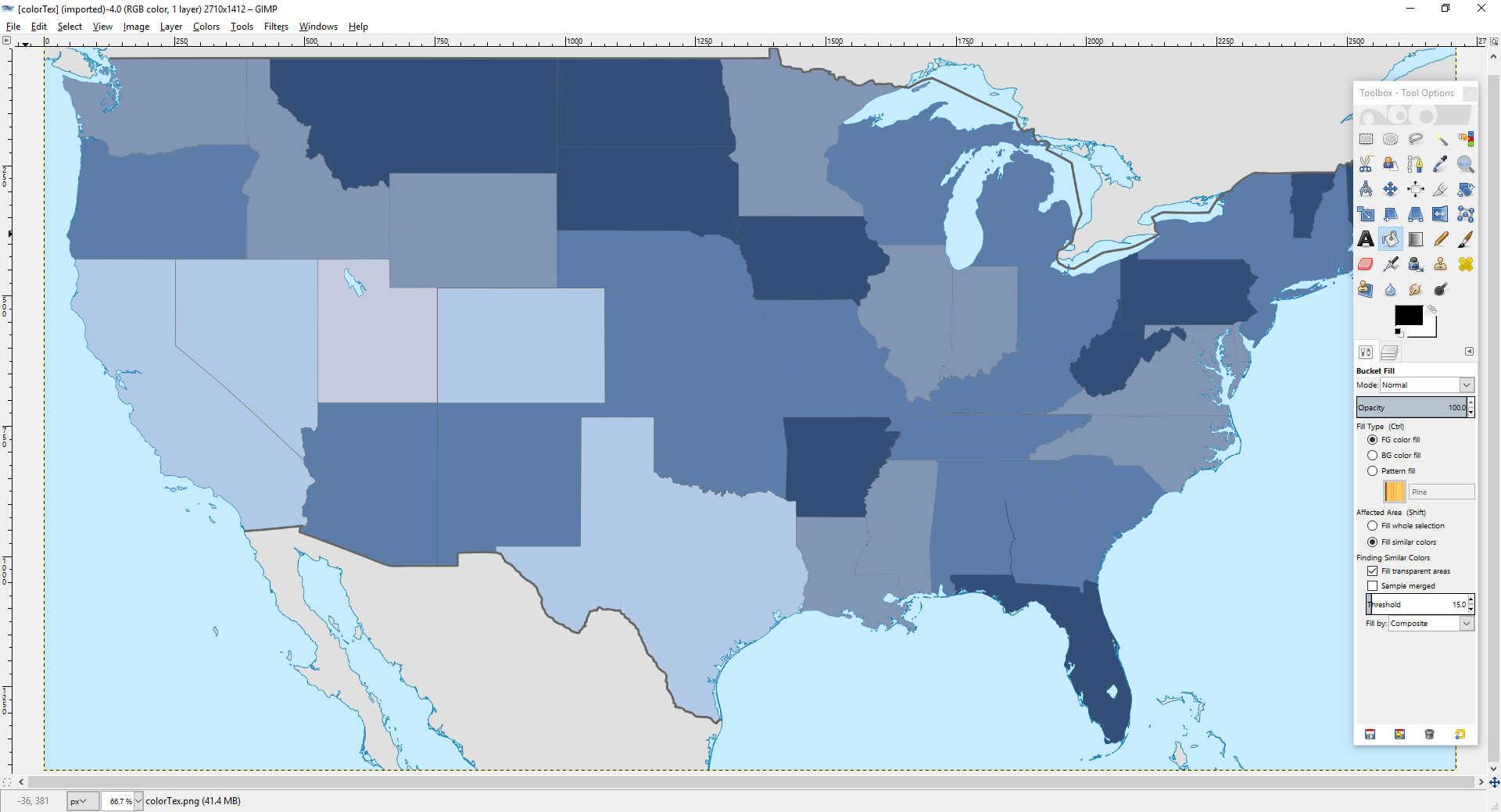
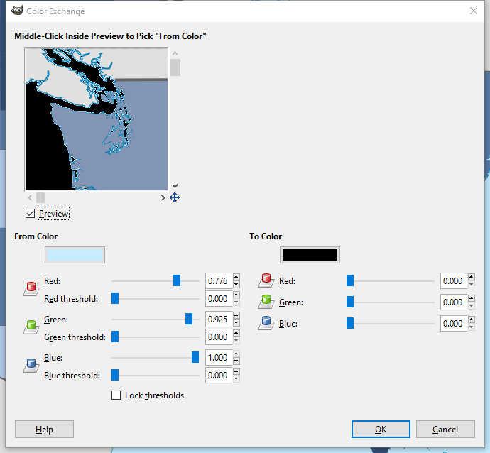
There are a few tools that will help create a heightmap from a color image in GIMP. In addition to the bucket fill, color picker and draw tools, we can also use the color exchange tool. This can be accessed in Colors→Map→Color Exchage. This allows you to quickly change all pixels of one color to another color. We can use this to set the color of all water pixels from their initial color to black. Similarly we can use this tool to set the color of "out of bounds" areas to black as well. We can also invert the color values pixels using Colors→Invert or Colors→Value Invert. The first of these inversion tools inverts the red, green, and blue values of all the pixels in the selected layer. The second just inverts the value of each pixel in the selected layer and keeps the hue and saturation of each pixel the same. For a black and white image these two are equivalent. These tools are great when the color map on your image is such that higher values are represented by darker colors, which is the case with the color map of the infographic above.

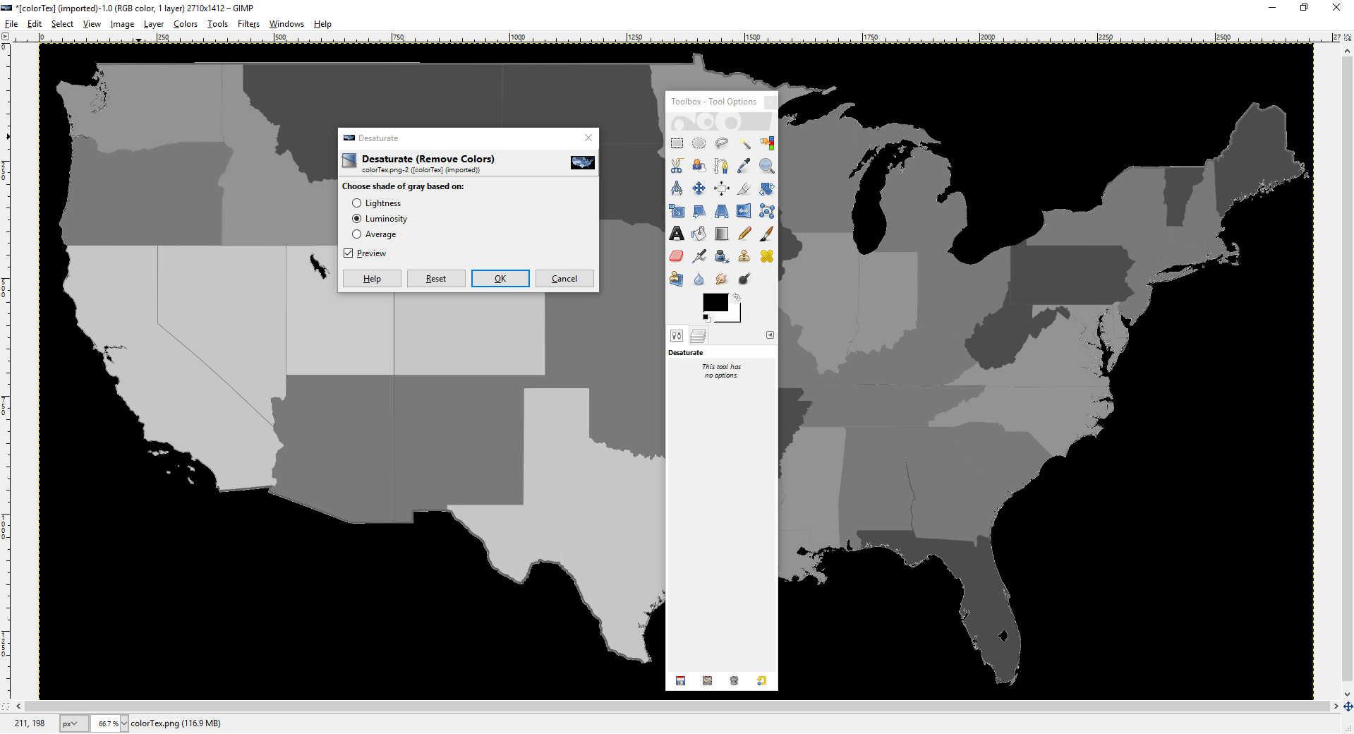
Another useful tool that we can use is the desaturation tool Colors→Desaturate. This tool provides a few different ways to convert the color values into grayscale values, which is what we want for the heightmap. "Lightness" transforms the pixel based on the average of the minimum and maximum of a pixels red, green and blue values. "Lightness" calculates a weighted average of the red, green, and blue values that is heavily biased towards the green value. "Average" calculates a grayscale value that is the unweighted average of the red, green, and blue values. You can preview the desaturation effect before you apply it, and see which version gives you the best result.

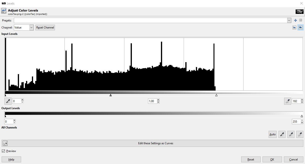
There are also multiple ways to change the distribution of color or grayscale values. In general, we would want to use the full range of grayscale values available. If we just want to perform a linear rescaling of the grayscale values we can use the Colors→Levels tool. In this tool menu, we can see a histogram of the value of each pixel and can move to sliders or enter the appropriate values to map the desired input range to the desired output range. If you want to apply a general transformation on the value of each pixel you can use Colors→Curves. This tool lets you draw the transformation function for the pixel values. For both tools, you can preview the transformations before you apply them to the image